
A cloud playout quote says $72 for a channel running continuously in a 30-day month. A second quote puts live video processing alone above $2,800 for the same number of hours. Both figures can be reasonable. The first may cover a schedule and a manifest assembled from prepared files. The second can include two live inputs, five output renditions, and advanced audio processing.
Cloud playout economics start with a clear endpoint. If the business needs a finished linear output with graphics, regional substitutions, and a tested fallback, an assembly price is one line of the budget. If it needs a pop-up channel built from already packaged content, paying for a pair of always-on encoders can make the same comparison misleading in the other direction.
What are you buying when a vendor quotes cloud playout?
Start with the signal the receiver should get, then trace backward to the source. A linear broadcaster may require an output delivered to affiliates in a specified transport, with captions, audio variants, graphics, break signaling, and continuous operation. A free ad-supported streaming television service assembled from prepared content may need a program schedule, adaptive playback, a guide, and ad opportunities at defined breaks. A quote covering either can accurately say channel.
Function | Ask the supplier to price | Verify at the handoff |
|---|---|---|
Scheduling and source selection | Schedule engine, live overrides, regional versions and operator seats | A late change appears on the intended output at the correct time. |
Live processing | Input, graphics, audio, captions, encoding and every output rendition | The receiver can decode the required media and signaling. |
Distribution | Contribution paths, packaging, origin, carriage and internet delivery where applicable | All destination feeds work during a route or origin failure. |
Recovery and operations | Standby, duplicate connectivity, monitoring, on-call and rehearsals | A named operator can restore service inside the required recovery time. |
Exit | Schedule and asset exports, configuration, overlap and cutback | A replacement system can take over with the expected schedule and rights intact. |
The question to put on every request for quotation is simple: at what point in the chain does your price stop? Draw that boundary across both designs. A service that stops at a primary origin should carry the same downstream costs as an on-premises design that stops there. If they route differently, price the differences and carry the common costs visibly outside the comparison.
A second diagram should show the backup path. It may use the same scheduler, storage origin, identity provider, contribution circuit, or delivery partner as the primary. Two running channels in different locations offer limited protection when the same dependency can take down both. Match designs on the failures they must withstand before comparing their price per hour.
What do public cloud rates actually cover?
AWS Elemental MediaTailor’s US East (Northern Virginia) examples list $0.10 per running hour for basic Channel Assembly and $0.35 for standard. Basic schedules video on demand. Standard can schedule prepared and live sources. The MediaTailor documentation describes assembling a live manifest from existing source manifests. Source encoding, storage, delivery, and monetization can add separate charges depending on the design. At 720 hours, the stated hourly rates give $72 and $252 respectively. These are component costs in U.S. dollars at rates checked November 6, 2026.
For a live processing example in the same region, AWS publishes an on-demand MediaLive standard channel at $3.942 per hour with two HD inputs, five output renditions, and advanced audio. Running 720 hours at that rate costs $2,838.24 for that configuration. AWS describes a standard MediaLive channel as two processing pipelines in different Availability Zones within a region. Cross-region recovery requires a separate design and budget. The channel can incur charges while running even when its inputs are idle. AWS also offers reserved pricing, which commits spending for the term even when schedules change.
The examples cover different functions and neither is a managed playout bid. Quote the live encoder only where the design requires it. Apply the assembly rate only to a design that uses that service. A broadcaster may already own one stage or buy it through a partner. Include the marginal cost and any capacity it would displace. If a quote says a stage is included, verify the number of supported channels, formats, and outputs before assigning it a zero in the comparison.
How do active channel hours change the break-even?
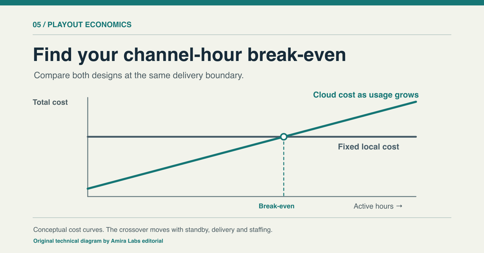
Cloud can be attractive for occasional channels when the active workload scales down after a show. Local infrastructure can be attractive when a stable schedule fills capacity you already own or can buy at a favorable monthly cost. Write the monthly cost of each design as fixed cost plus variable cost per active hour times aggregate active channel hours. Twelve channels running 80 hours each create 960 active channel-hours. Capacity still has to support the busiest simultaneous hour.
Assume a cloud design has $1,200 in monthly fixed costs and an average variable cost of $4.20 per active channel-hour. Assume a local design has $12,000 in monthly fixed costs and $0.60 per active channel-hour. These are hypothetical, fully specified comparison inputs, independent of the AWS component examples. Assume both meet the same operating requirements and the local setup can handle all 12 channels concurrently. Carry any comparable, identical downstream cost outside both totals.
Active hours per channel across 12 channels | Aggregate hours | Cloud | Local |
|---|---|---|---|
80 | 960 | $5,232 | $12,576 |
250 | 3,000 | $13,800 | $13,800 |
720 | 8,640 | $37,488 | $17,184 |
The fixed-cost difference is $10,800 and the hourly difference is $3.60. Dividing gives a crossover at 3,000 active channel-hours per month, or 250 hours per channel if they are evenly scheduled. The dividing formula applies here because the local design has a higher fixed cost and a lower variable cost. If one design costs less on both measures, there is no positive crossover under the model. If you need a second equipment purchase at peak concurrency, or a cloud commitment makes some of the bill payable regardless of use, use a separate cost curve for each capacity or pricing tier.
Define active from the invoice and the runbook. A two-hour match may keep live infrastructure ready for rehearsal, pregame, overtime, and postgame. Standby and warmup can consume billable hours even if a viewer never sees the slate. If the quote assumes resources shut down between events, rehearse a cold start and record how much setup time has to be purchased. If the supplier requires capacity reserved for every game day, carry that reserve as fixed spend or contracted hours.
Which costs can move the crossover the most?
Persistent delivery, standby, and staffing can outweigh the variable processor rate. At an illustrative 8 megabits per second, one unbroken output carries 3.6 decimal GB per hour. Twelve such outputs running for 720 hours carry about 31.1 TB across a single metered leg. A second full-rate copy over a separately billed path adds another 31.1 TB. These are transfer volumes before overhead. They exclude consumer streaming traffic, which depends on audience, playback bitrate, and caching.
Use the route map to identify which paths charge by volume, by reserved throughput, or by a fixed circuit fee. AWS Elemental MediaConnect pricing, for example, describes running transport-flow charges plus relevant transfer charges and a reserved outbound bandwidth option. For an audience-facing service, build a separate viewer delivery estimate and include it where the location decision changes it. Keep an affiliate transport feed and consumer content delivery network traffic on distinct rows.
Staffing can also shift the calculation. Ask who makes a late schedule change, who switches to backup, and who can escalate a corrupted asset at night. A managed contract may include some of that work. The customer can still own the handoff to affiliates or a decision about rights. Count the incremental staff hours each design needs, then separate them from people who remain on the payroll in either case. Do the same for space, power, spares, licenses, network circuits, and depreciation or financing. For an installed plant, show both the short-term avoidable cost and the cost at the next refresh. The investment decision can differ across those horizons.
When does a lower monthly cost fail the operating test?
A cheaper design fails when it cannot deliver the required signal or recover on the agreed clock. A sports channel that relies on local intervention for an unplanned break needs a tested control path from the person on duty to the live output. A replacement schedule service needs the right rights windows, identifiers, regional rules, and access to the original material. Add an overlap period and an exit exercise to the business case so a lower monthly quote does not hide the cost of moving in either direction.
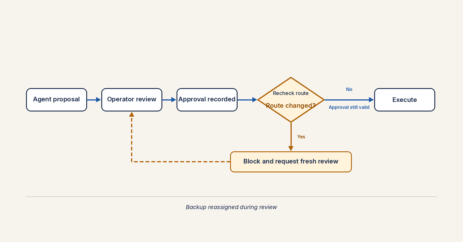
Use a representative failure. Disconnect one input or route while a late schedule change is in flight. Verify what viewers and downstream receivers actually see. Measure how long it takes to detect the failure, take the backup, and restore normal service. Ask a second operator to repeat the recovery without the installation team. The managed playout verification guide gives engineers a way to document those handoffs and preserve independent evidence.
The cost comparison can be especially sensitive at modest scale. A small station that lacks a staffed backup site may pay more for on-premises recovery than its first quote suggests. A large group with existing shared facilities may be able to absorb steady channels into available capacity. In either case, price the minimum service that passes the same test and rerun the comparison at the next material step in capacity.
What should go into the procurement worksheet this week?
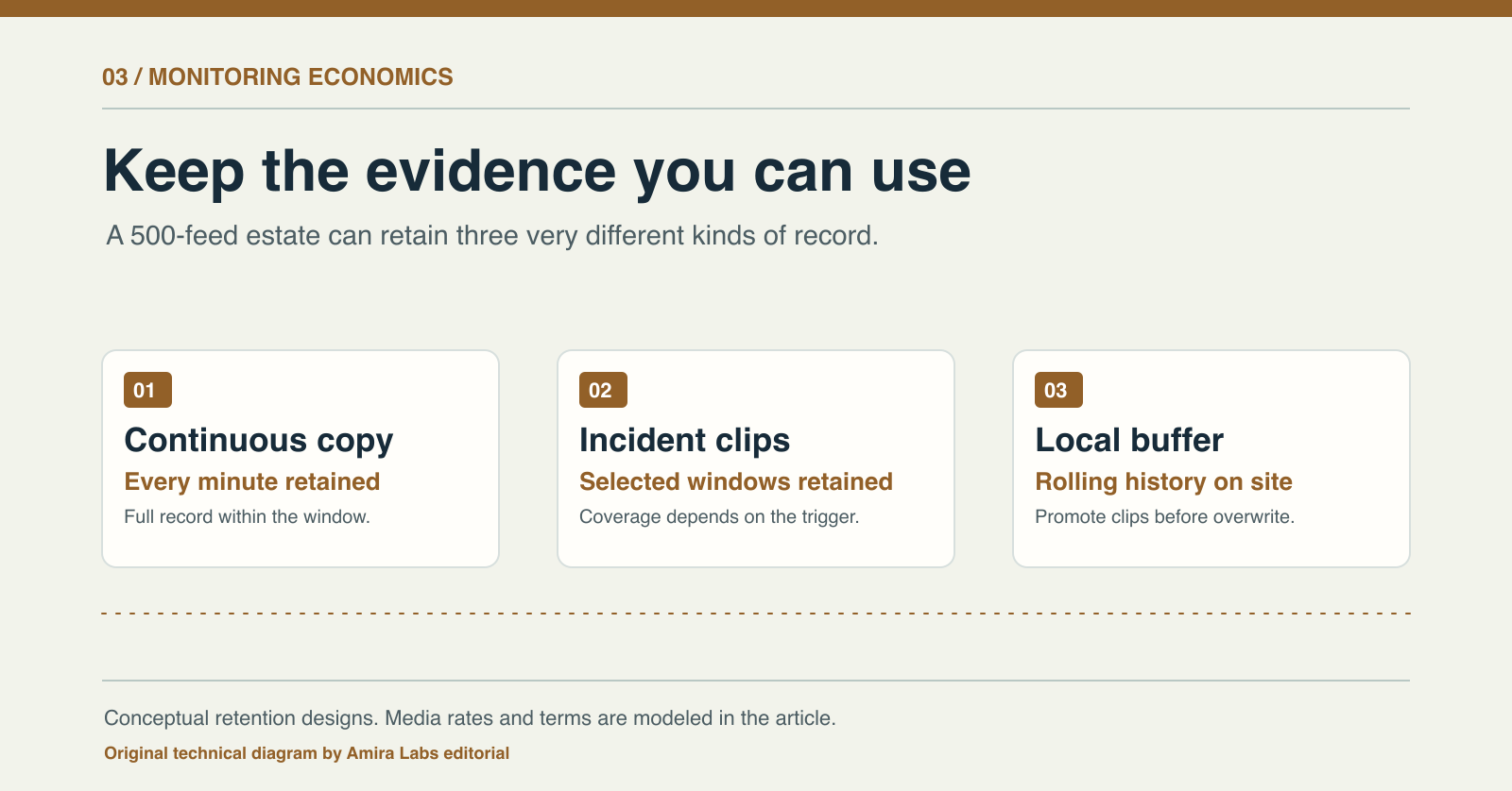
Export the last representative month of schedules and mark continuous channels, occasional events, rehearsals, and regional forks. Count active hours and peak concurrency separately. For each delivery path, record the bitrate, how many copies cross a paid boundary, and which party pays. Ask suppliers to separate committed, active, and standby hours on the same worksheet.
Use one test channel to verify a cold start, a late schedule change, and the loss of a primary path. Bring the measured startup time and recovery staffing back into the monthly model. Then price the next refresh or renewal and a month when the schedule is unusually busy. The crossover you can defend is the one that reflects a channel you have actually taken to air under the required conditions.
Sources
- AWS Elemental MediaTailor pricing, US East (Northern Virginia) Channel Assembly examples, checked November 6, 2026
- AWS Elemental MediaTailor, Channel Assembly source and manifest workflow, checked November 6, 2026
- AWS Elemental MediaLive pricing and US East (Northern Virginia) on-demand standard example, checked November 6, 2026
- AWS Elemental MediaConnect pricing and transfer dimensions, checked November 6, 2026